Introduction
Recently, when helping a user who wanted to compute centroids from vectors held in ClickHouse, we realized that the same solution could be used to implement K-Means clustering. They wanted to solve this at scale across potentially billions of data points while ensuring memory could be tightly managed. In this post, we give implementing K-means clustering using just SQL a try and show that it scales to billions of rows.
In the writing of this blog, we became aware of the work performed by Boris Tyshkevich. While we use a different approach in this blog, we would like to recognize Boris for his work and for having this idea well before we did!
As part of implementing K-Means with ClickHouse SQL, we cluster 170M NYC taxi rides in under 3 minutes. The equivalent scikit-learn operation with the same resources takes over 100 minutes and requires 90GB of RAM. With no memory limitations and ClickHouse automatically distributing the computation, we show that ClickHouse can accelerate machine learning workloads and reduce iteration time.
All of the code for this blog post can be found in a notebook here.
Why K-Means in ClickHouse SQL?
The key motivation for using ClickHouse SQL to do K-Means is that training is not memory-bound, making it possible to cluster PB datasets thanks to the incremental computation of centroids (with settings to limit memory overhead). In contrast, distributing this workload across servers using Python-based approaches would require an additional framework and complexity.
Additionally, we can easily increase the level of parallelism in our clustering to use the full resources of a Clickhouse instance. Should we need to handle larger datasets, we simply scale the database service - a simple operation in ClickHouse Cloud.
Transforming the data for K-Means is a simple SQL query that can process billions of rows per second. With centroids and points held in ClickHouse, we can compute statistics such as model errors with just SQL and potentially use our clusters for other operations e.g. product quantization for vector search.
K-Means recap
K-Means is an unsupervised machine learning algorithm for partitioning a dataset into K distinct, non-overlapping subgroups (clusters) where each data point belongs to the cluster with the nearest mean (the cluster's centroid). The process begins by initializing K centroids randomly or based on some heuristic. These centroids serve as the initial representatives of the clusters. The algorithm then iterates through two main steps until convergence: assignment and update.
In the assignment step, each data point is assigned to the nearest cluster based on the Euclidean distance (or another distance metric) between it and the centroids. In the update step, the centroids are recalculated as the mean of all points assigned to their respective clusters, potentially shifting their positions.
This process is guaranteed to converge, with the assignments of points to clusters eventually stabilizing and not changing between iterations. The number of clusters, K, needs to be specified beforehand and heavily influences the algorithm's effectiveness with the optimal value depending on the dataset and the goal of the clustering. For more details, we recommend this excellent overview.
Points and centroids
The key problem our user posed was the ability to efficiently compute centroids. Suppose we have a simple data schema for a transactions table, where each row represents a bank transaction for a specific customer. Vectors in ClickHouse are represented as an Array type.
CREATE TABLE transactions
(
  id UInt32,
  vector Array(Float32),
  -- e.g.[0.6860357,-1.0086979,0.83166444,-1.0089169,0.22888935]
  customer UInt32,
  ...other columns omitted for brevity
)
ENGINE = MergeTree ORDER BY id
Our user wanted to find the centroid for each customer, effectively the positional average of all the transaction vectors associated with each customer. To find the set of average vectors, we can use the avgForEach[1][2] function. For instance, consider the example of computing the average of 3 vectors, each with 4 elements:
WITH vectors AS
   (
       SELECT c1 AS vector
       FROM VALUES([1, 2, 3, 4], [5, 6, 7, 8], [9, 10, 11, 12])
   )
SELECT avgForEach(vector) AS centroid
FROM vectors

┌─centroid──┐
│ [5,6,7,8] │
└───────────┘
In our original transactions table, computing the average per customer thus becomes:
SELECT customer, avgForEach(vector) AS centroid FROM transactions GROUP BY customer
While simple, this approach has a few limitations. Firstly, for very large datasets, when the vector contains many Float32 points and the customer column has many unique elements (high cardinality), this query can be very memory intensive. Secondly, and maybe more relevant to K-Means, this approach requires us to rerun the query if new rows are inserted, which is inefficient. We can address these problems through Materialized Views and the AggregatingMergeTree engine.
Incrementally computing centroids with Materialized Views
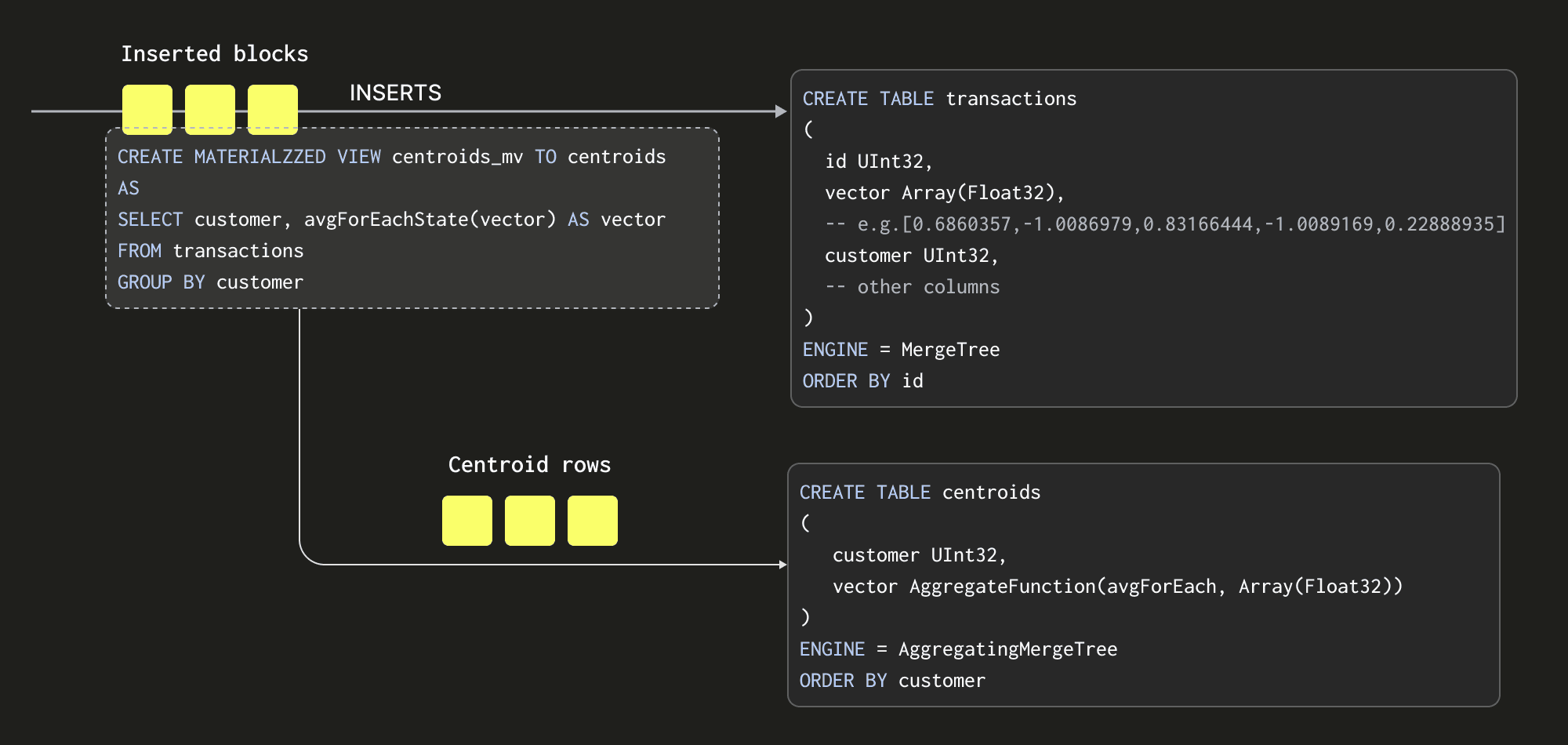
Materialized Views allow us to shift the cost of computing our centroids to insert time. Unlike in other databases, a ClickHouse Materialized View is just a trigger that runs a query on blocks of data as they are inserted into a table. The results of this query are inserted into a second "target" table. In our case, the Materialized View query will compute our centroids, inserting the results to a table centroids.
There are some important details here:
- Our query, which computes our centroids, must produce the result set in a format that can be merged with subsequent result sets - since every block inserted will produce a result set. Rather than just sending averages to our
centroidstable (the average of an average would be incorrect), we send the “average state”. The average state representation contains the sum of each vector position, along with a count. This is achieved using theavgForEachStatefunction - notice how we’ve just appendedStateto our function name! The AggregatingMergeTree table engine is required to store these aggregation states. We explore this more below. - The entire process is incremental with the
centroidstable containing the final state i.e. a row per centroid. Readers will notice that the table which receives inserts has a Null table engine. This causes the inserted rows to be thrown away, saving the IO associated with writing the full dataset on each iteration. - The query of our Materialized View is only executed on the blocks as they are inserted. The number of rows in each block can vary depending on the method of insertion. We recommend at least 1000 rows per block if formulating blocks on the client side, e.g., using the Go client. If the server is left to form blocks (e.g. when inserting by HTTP), the size can also be specified.
- If using an
INSERT INTO SELECTwhere ClickHouse reads rows from another table or external source, e.g. S3, the block size can be controlled by several key parameters discussed in detail in previous blogs. These settings (along with the number of insert threads) can have a dramatic effect on both the memory used (larger blocks = more memory) and the speed of ingestion (larger blocks = faster). These settings mean the amount of memory used can be finely controlled in exchange for performance.
AggregatingMergeTree
Our target table centroids uses the engine AggregatingMergeTree:
CREATE TABLE centroids
(
   customer UInt32,
   vector AggregateFunction(avgForEach, Array(Float32))
)
ENGINE = AggregatingMergeTree  ORDER BY customer
Our vector column here contains the aggregate states produced by the avgForEachState function above. These are intermediate centroids that must be merged to produce a final answer. This column needs to be of the appropriate type AggregateFunction(avgForEach, Array(Float32)).
Like all ClickHouse MergeTree tables, the AggregatingMergeTree stores data as parts that must be merged transparently to allow more efficient querying. When merging parts containing our aggregate states, this must be done so that only states pertaining to the same customer are merged. This is effectively achieved by ordering the table by the customer column with the ORDER BY clause. At query time, we must also ensure intermediate states are grouped and merged. This can be achieved by ensuring we GROUP BY by the column customer and use the Merge equivalent of the avgForEach function: avgForEachMerge.
SELECT customer, avgForEachMerge(vector) AS centroid
FROM centroids GROUP BY customer
All aggregation functions have an equivalent state function, obtained by appending
Stateto their name, which produces an intermediate representation that can be stored and then retrieved and merged with aMergeequivalent. For more details, we recommend this blog and the video from our very own Mark.
This query will be very fast compared to our earlier GROUP BY. Most of the work for computing averages has been moved to insert time, with a small number of rows left for query time merging. Consider the performance of the following two approaches using 100m random transactions on a 48GiB, 12 vCPU Cloud service. Steps to load the data here.
Contrast the performance of computing our centroids from the transactions table:
SELECT customer, avgForEach(vector) AS centroid
FROM transactions GROUP BY customer
ORDER BY customer ASC
LIMIT 1 FORMAT Vertical

10 rows in set. Elapsed: 147.526 sec. Processed 100.00 million rows, 41.20 GB (677.85 thousand rows/s., 279.27 MB/s.)

Row 1:
──────
customer: 1
centroid: [0.49645231463677153,0.5042792240640065,...,0.5017436349466129]

1 row in set. Elapsed: 36.017 sec. Processed 100.00 million rows, 41.20 GB (2.78 million rows/s., 1.14 GB/s.)
Peak memory usage: 437.54 MiB.
vs the centroids table with is over 1700x faster:
SELECT customer, avgForEachMerge(vector) AS centroid
FROM centroids GROUP BY customer
ORDER BY customer ASC
LIMIT 1
FORMAT Vertical

Row 1:
──────
customer: 1
centroid: [0.49645231463677153,0.5042792240640065,...,0.5017436349466129]

1 row in set. Elapsed: 0.085 sec. Processed 10.00 thousand rows, 16.28 MB (117.15 thousand rows/s., 190.73 MB/s.)
Putting it all together
With our ability to compute centroids incrementally, let's focus on K-Means clustering. Let's assume we're trying to cluster a table points where each row has a vector representation. Here, we will cluster on similarity rather than just basing our centroids on the customer as we did with transactions.
A single iteration
We need to be able to store the current centroids after each iteration of the algorithm. For now, let's assume we have identified an optimal value of K. Our target table for our centroids might look like this:
CREATE TABLE centroids
(
  k UInt32,
  iteration UInt32,
  centroid UInt32,
  vector AggregateFunction(avgForEach, Array(Float32))
)
ENGINE = AggregatingMergeTree
ORDER BY (k, iteration, centroid)
The value of the k column is set to our chosen value of K. Our centroid column here denotes the centroid number itself, with a value between 0 and K-1. Rather than use a separate table for each iteration of the algorithm, we simply include an iteration column and ensure our ordering key is (k, iteration, centroid). ClickHouse will ensure the intermediate state is only merged for each unique K, centroid, and iteration. This means our final row count will be small, ensuring fast querying of these centroids.
Our Materialized View for computing our centroids should be familiar with only a small adjustment to also GROUP BY k, centroid, and iteration:
CREATE TABLE temp
(
   k UInt32,
   iteration UInt32,
   centroid UInt32,
   vector Array(Float32)
)
ENGINE = Null

CREATE MATERIALIZED VIEW centroids_mv TO centroids
AS SELECT k, iteration, centroid, avgForEachState(vector) AS vector
FROM temp GROUP BY k, centroid, iteration
Notice that our query executes over blocks inserted into a temp table, not our data source table transactions, which does not have an iteration or centroid column. This temp table will receive our inserts and uses the Null table engine again to avoid writing data. With these building blocks in place, we can visualize a single iteration of the algorithm assuming K = 5:
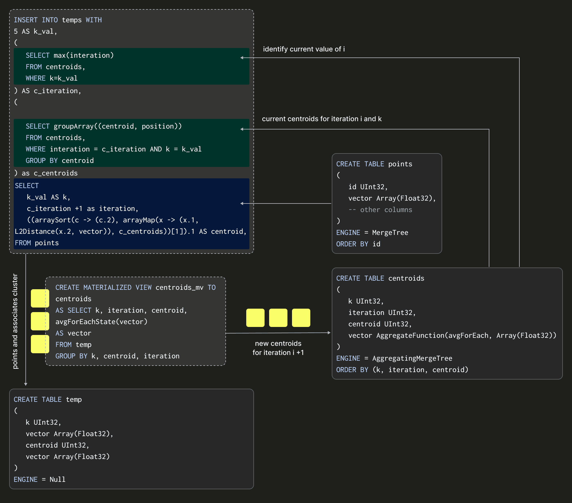
The above shows how we insert into our temp table and thus compute our centroids by performing an INSERT INTO SELECT with a points table as our source data. This insertion effectively represents an iteration of the algorithm. The SELECT query here is critical as it needs to specify the transaction vector and its current centroid and iteration (and fixed value of K). How might we compute the latter of these two? The full INSERT INTO SELECT is shown below:
INSERT INTO temp
WITH
  5 as k_val,
  -- (1) obtain the max value of iteration - will be the previous iteration
  (
      SELECT max(iteration)
      FROM centroids
      -- As later we will reuse this table for all values of K
      WHERE k = k_val
  ) AS c_iteration,
  (
      -- (3) convert centroids into a array of tuples
      -- i.e. [(0, [vector]), (1, [vector]), ... , (k-1, [vector])]
      SELECT groupArray((centroid, position))
      FROM
      (
         -- (2) compute the centroids from the previous iteration
          SELECT
              centroid,
              avgForEachMerge(vector) AS position
          FROM centroids
          WHERE iteration = c_iteration AND k = k_val
          GROUP BY centroid
      )
  ) AS c_centroids
SELECT
  k_val AS k,
  -- (4) increment the iteration
  c_iteration + 1 AS iteration,
  -- (5) find the closest centroid for this vector using Euclidean distance
  (arraySort(c -> (c.2), arrayMap(x -> (x.1, L2Distance(x.2, vector)), c_centroids))[1]).1 AS centroid,
  vector AS v
FROM points
Firstly, at (1), this query identifies the number of the previous iteration. This is then used within the CTE at (2) to determine the centroids produced for this iteration (and chosen K), using the same avgForEachMerge query shown earlier. These centroids are collapsed into a single row containing an array of Tuples via the groupArray query to facilitate easy matching against the points. In the SELECT, we increment the iteration number (4) and compute the new closest centroid (with the Euclidean distance L2Distance function) using an arrayMap and arraySort functions for each point.
By inserting the rows into temp here, with a centroid based on the previous iteration, we can allow the Materialized View to compute the new centroids (with the iteration value +1).
Initializing the centroids
The above assumes we have some initial centroids for iteration 1, which are used to compute membership. This requires us to initialize the system. We can do this by simply selecting and inserting K random points with the following query (k=5):
INSERT INTO temp WITH
  5 as k_val,
  vectors AS
  (
      SELECT vector
      FROM points
      -- select random points, use k to make pseudo-random
      ORDER BY cityHash64(concat(toString(id), toString(k_val))) ASC
      LIMIT k_val -- k
  )
SELECT
  k_val as k,
  1 AS iteration,
  rowNumberInAllBlocks() AS centroid,
  vector
FROM vectors
Successful clustering is very sensitive to the initial placement of centroids; poor assignment leads to slow convergence or suboptimal clustering. We will discuss this a little later.
Centroid assignment and when to stop iterating
All of the above represents a single iteration (and initialization step). After each iteration, we need to make a decision as to whether to stop based on an empirical measurement of whether the clustering has converged. The simplest way to do this is to simply stop when points no longer change centroids (and thus clusters) between iterations.
To identify which points belong to which centroids, we can use the above SELECT from our earlier
INSERT INTO SELECTat any time.
To compute the number of points that moved clusters in the last iteration, we first compute the centroids for the previous two iterations (1) and (2). Using these, we identify the centroids for each point for each iteration (3) and (4). If these are the same (5), we return 0 and 1 otherwise. A total of these (6) values provides us with the number of points that moved clusters.
WITH 5 as k_val,
(
      SELECT max(iteration)
      FROM centroids
) AS c_iteration,
(
  -- (1) current centroids
  SELECT groupArray((centroid, position))
  FROM
  (
      SELECT
          centroid,
          avgForEachMerge(vector) AS position
      FROM centroids
      WHERE iteration = c_iteration AND k = k_val
      GROUP BY centroid
  )
) AS c_centroids,
(
  -- (2) previous centroids
  SELECT groupArray((centroid, position))
  FROM
  (
      SELECT
          centroid,
          avgForEachMerge(vector) AS position
      FROM centroids
      WHERE iteration = (c_iteration-1) AND k = k_val
      GROUP BY centroid
  )
) AS c_p_centroids
-- (6) sum differences
SELECT sum(changed) FROM (
  SELECT id,
  -- (3) current centroid for point
  (arraySort(c -> (c.2), arrayMap(x -> (x.1, L2Distance(x.2, vector)), c_centroids))[1]).1 AS cluster,
  -- (4) previous centroid for point
  (arraySort(c -> (c.2), arrayMap(x -> (x.1, L2Distance(x.2, vector)), c_p_centroids))[1]).1 AS cluster_p,
  -- (5) difference in allocation
  if(cluster = cluster_p, 0, 1) as changed
  FROM points
)
A test dataset
The above has been mostly theoretical. Let's see if the above actually works on a real dataset! For this, we'll use a 3m row subset of the popular NYC taxis dataset as the clusters are hopefully relatable. To create and insert the data from S3:
CREATE TABLE trips (
  trip_id         	UInt32,
  pickup_datetime 	DateTime,
  dropoff_datetime	DateTime,
  pickup_longitude	Nullable(Float64),
  pickup_latitude 	Nullable(Float64),
  dropoff_longitude   Nullable(Float64),
  dropoff_latitude	Nullable(Float64),
  passenger_count 	UInt8,
  trip_distance   	Float32,
  fare_amount     	Float32,
  extra           	Float32,
  tip_amount      	Float32,
  tolls_amount    	Float32,
  total_amount    	Float32,
  payment_type    	Enum('CSH' = 1, 'CRE' = 2, 'NOC' = 3, 'DIS' = 4, 'UNK' = 5),
  pickup_ntaname  	LowCardinality(String),
  dropoff_ntaname 	LowCardinality(String)
)
ENGINE = MergeTree
ORDER BY (pickup_datetime, dropoff_datetime);

INSERT INTO trips SELECT trip_id, pickup_datetime, dropoff_datetime, pickup_longitude, pickup_latitude, dropoff_longitude, dropoff_latitude, passenger_count, trip_distance, fare_amount, extra, tip_amount, tolls_amount, total_amount, payment_type, pickup_ntaname, dropoff_ntaname
FROM gcs('https://storage.googleapis.com/clickhouse-public-datasets/nyc-taxi/trips_{0..2}.gz', 'TabSeparatedWithNames');
Feature selection
Feature selection is crucial for good clustering as it directly impacts the quality of the clusters formed. We won’t go into detail here on how we selected our features. For those interested, we include the notes in the notebook. We end up with the following points table:
CREATE TABLE points
(
   `id` UInt32,
   `vector` Array(Float32),
   `pickup_hour` UInt8,
   `pickup_day_of_week` UInt8,
   `pickup_day_of_month` UInt8,
   `dropoff_hour` UInt8,
   `pickup_longitude` Float64,
   `pickup_latitude` Float64,
   `dropoff_longitude` Float64,
   `dropoff_latitude` Float64,
   `passenger_count` UInt8,
   `trip_distance` Float32,
   `fare_amount` Float32,
   `total_amount` Float32
) ENGINE = MergeTree ORDER BY id
To populate this table, we use an INSERT INTO SELECT SQL query, which creates the features, scales them, and filters any outliers. Note our final columns are also encoded in a vector column.
The linked query is our first attempt at producing features. We expect more work to be possible here, which might produce better results than those shown. Suggestions are welcome!
A little bit of Python
We have described how an iteration in the algorithm effectively reduces to an INSERT INTO SELECT, with the Materialized View handling the maintenance of the centroids. This means we need to invoke this statement N times until convergence has occurred.
Rather than waiting to reach a state where no points move between centroids, we use a threshold of 1000 i.e. if fewer than 1000 points move clusters, we stop. This check is made every 5 iterations.
The pseudo code for performing K-Means for a specific value of K becomes very simple given most of the work is performed by ClickHouse.
def kmeans(k, report_every = 5, min_cluster_move = 1000):
   startTime = time.time()
   # INITIALIZATION QUERY
   run_init_query(k)
   i = 0
   while True:
       # ITERATION QUERY
       run_iteration_query(k)
       # report every N iterations
       if (i + 1) % report_every == 0 or i == 0:
           num_moved = calculate_points_moved(k)
           if num_moved <= min_cluster_move:
               break
       i += 1
   execution_time = (time.time() - startTime))
   # COMPUTE d^2 ERROR
   d_2_error = compute_d2_error(k)
   # return the d^2, execution time and num of required iterations
   return d_2_error, execution_time, i+1
The full code for this loop, including the queries, can be found in the notebook.
Choosing K
So far, we’ve assumed K has been identified. There are several techniques for determining the optimal value of K, the simplest of which is to compute the aggregate squared distance (SSE) between each point and its respective cluster for each value of K. This gives us a cost metric that we aim to minimize. The method compute_d2_error computes this using the following SQL query (assuming a value of 5 for K):
WITH 5 as k_val,
(
       SELECT max(iteration)
       FROM centroids WHERE k={k}
) AS c_iteration,
(
   SELECT groupArray((centroid, position))
   FROM
   (
       SELECT
           centroid,
           avgForEachMerge(vector) AS position
       FROM centroids
       WHERE iteration = c_iteration AND k=k_val
       GROUP BY centroid
   )
) AS c_centroids
SELECT
   sum(pow((arraySort(c -> (c.2), arrayMap(x -> (x.1, L2Distance(x.2, vector)), c_centroids))[1]).2, 2)) AS distance
FROM points
This value is guaranteed to decrease as we increase K e.g. if we set K to the number of points, each cluster will have 1 point thus giving us an error of 0. Unfortunately, this won’t generalize the data very well!
As K increases, SSE typically decreases because the data points are closer to their cluster centroids. The goal is to find the "elbow point" where the rate of decrease in SSE sharply changes. This point indicates a diminishing return on the benefit of increasing K. Choosing K at the elbow point provides a model that captures the inherent grouping in the data without overfitting. A simple way to identify this elbow point is to plot K vs SEE and identify the value visually. For our NYC taxis data, we measure and plot SSE for the K values 2 to 20:
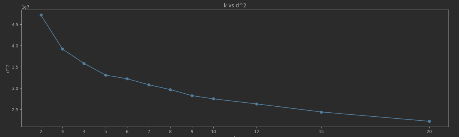
The elbow point here isn’t as clear as we’d like, but a value of 5 seems a reasonable candidate.
The above results are based on a single end-to-end run for each value of K. K-Means can converge to a local minimum with no guarantee that nearby points will end up in the same cluster. It would be advisable to run multiple values for each value of K, each time with different initial centroids, to find the best candidate.
Results
If we select 5 as our value for K, the algorithm takes around 30 iterations and 20 seconds to converge on a 12 vCPU ClickHouse Cloud node. This approach considers all 3 million rows for each iteration.
k=5
initializing...OK
Iteration 0
Number changed cluster in first iteration: 421206
Iteration 1, 2, 3, 4
Number changed cluster in iteration 5: 87939
Iteration 5, 6, 7, 8, 9
Number changed cluster in iteration 10: 3610
Iteration 10, 11, 12, 13, 14
Number changed cluster in iteration 15: 1335
Iteration 15, 16, 17, 18, 19
Number changed cluster in iteration 20: 1104
Iteration 20, 21, 22, 23, 24
Number changed cluster in iteration 25: 390
stopping as moved less than 1000 clusters in last iteration
Execution time in seconds: 20.79200577735901
D^2 error for 5: 33000373.34968858
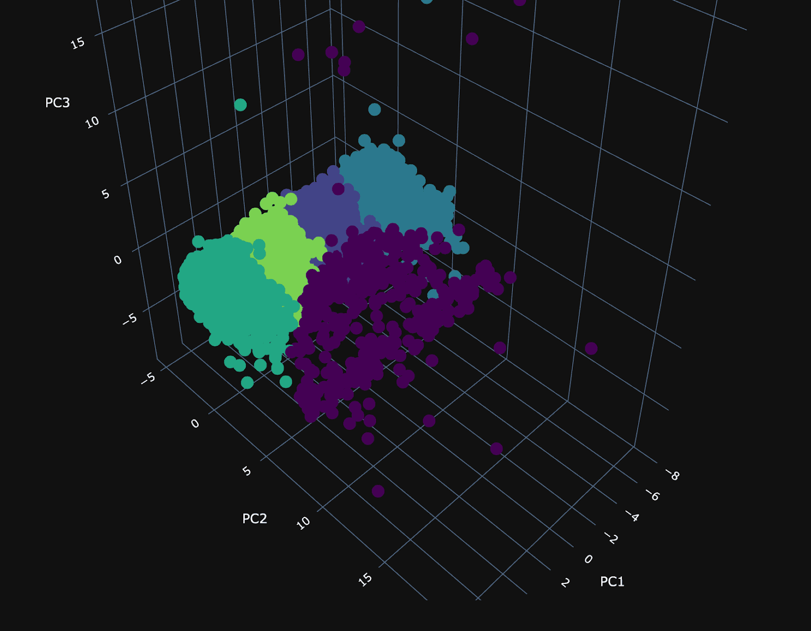
To visualize these clusters, we need to reduce the dimensionality. For this, we use Principal Component Analysis (PCA). We defer the implementation of PCA in SQL to another blog and just use Python with a sample of 10,000 random points. We can evaluate the effectiveness of PCA in capturing the essential properties of data by checking how much variance the principal components account for. 82% is less than the typically used threshold of 90%, but sufficient for an understanding of the effectiveness of our clustering:
Explained variances of the 3 principal components: 0.824
Using our 3 principal components, we can plot the same random 10,000 points and associate a color with each according to its cluster.
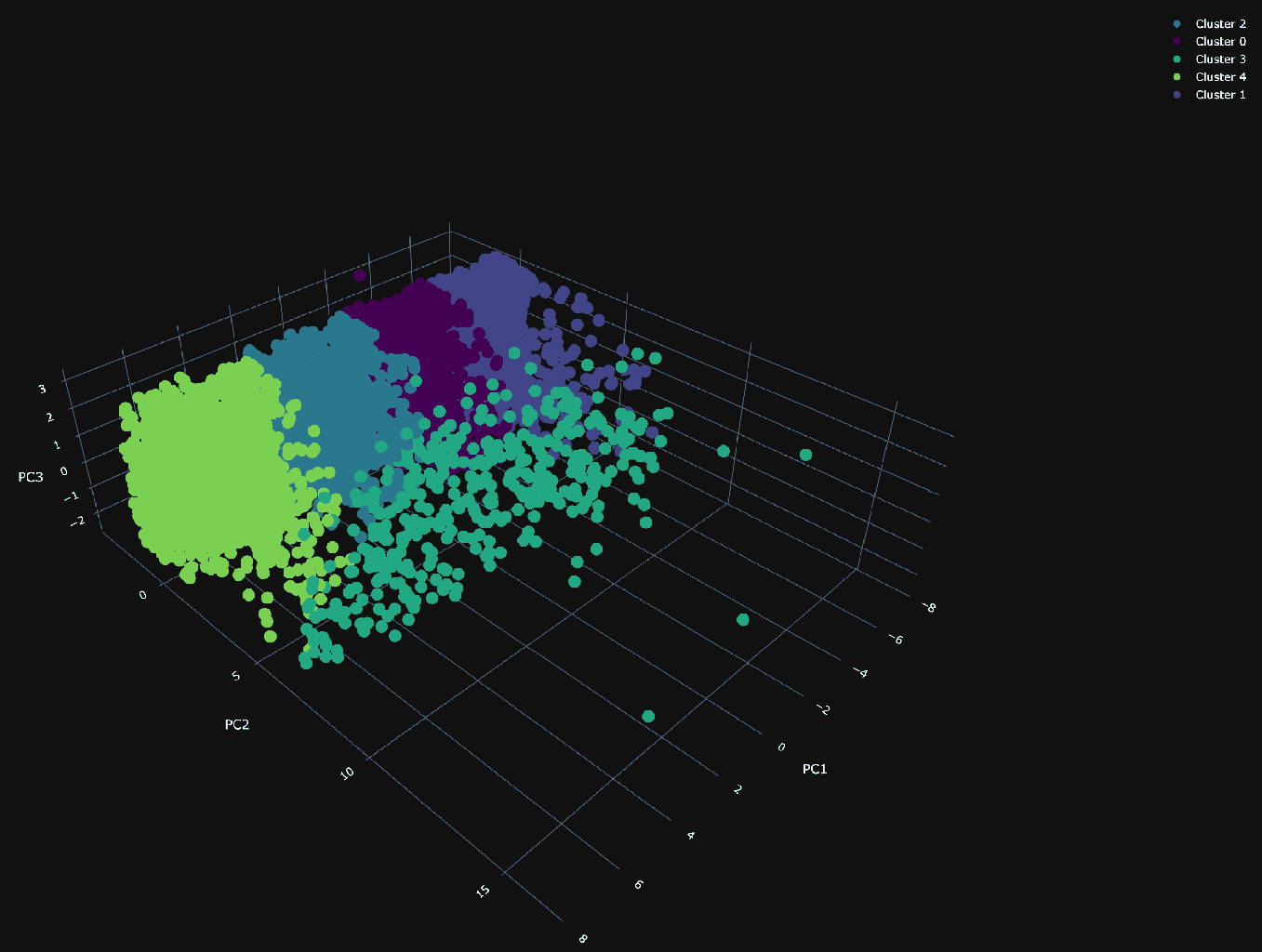
The PCA visualization of the clusters shows a dense plane across PC1 and PC3, neatly divided into four distinct clusters, suggesting constrained variance within these dimensions. Along the 2nd principal component (PC2), the visualization becomes sparser, with a cluster (number 3) that diverges from the main group and could be particularly interesting.
To understand our clusters, we need labels. Ideally, we would produce these by exploring the distribution of every column in each cluster, looking for unique characteristics and temporal/spatial patterns. We’ll try to do this succinctly with a SQL query to understand the distribution of each column in each cluster. For the columns to focus on, we can inspect the values of the PCA components and identify the dimensions that dominate. Code for doing this can be found in the notebook and identifies the following:
PCA1:: ['pickup_day_of_month: 0.9999497049810415', 'dropoff_latitude: -0.006371842399701939', 'pickup_hour: 0.004444108327647353', 'dropoff_hour: 0.003868258226185553', …]

PCA 2:: ['total_amount: 0.5489526881298809', 'fare_amount: 0.5463895585884886', 'pickup_longitude: 0.43181504878694826', 'pickup_latitude: -0.3074228612885196', 'dropoff_longitude: 0.2756342866763702', 'dropoff_latitude: -0.19809343490462433', …]

PCA 3:: ['dropoff_hour: -0.6998176337701472', 'pickup_hour: -0.6995098287872831', 'pickup_day_of_week: 0.1134719682173672', 'pickup_longitude: -0.05495391127067617', …]
For PCA1, pickup_day_of_month is important, suggesting a focus on the time of the month. For PC2, dimensions, the location of pickup and drop off, and the cost of the ride appear to contribute heavily. This component probably focuses on a specific trip type. Finally, for PC3, the hour in which the trip occurred seems the most relevant. To understand how these columns differ per cluster with respect to time, date, and price, we again can just use an SQL query:
WITH
   5 AS k_val,
   (
       SELECT max(iteration)
       FROM centroids
       WHERE k = k_val
   ) AS c_iteration,
   (
       SELECT groupArray((centroid, position))
       FROM
       (
           SELECT
               centroid,
               avgForEachMerge(vector) AS position
           FROM centroids
           WHERE (iteration = c_iteration) AND (k = k_val)
           GROUP BY centroid
       )
   ) AS c_centroids
SELECT
   (arraySort(c -> (c.2), arrayMap(x -> (x.1, L2Distance(x.2, vector)), c_centroids))[1]).1 AS cluster,
   floor(avg(pickup_day_of_month)) AS pickup_day_of_month,
   round(avg(pickup_hour)) AS avg_pickup_hour,
   round(avg(fare_amount)) AS avg_fare_amount,
   round(avg(total_amount)) AS avg_total_amount
FROM points
GROUP BY cluster
ORDER BY cluster ASC

┌─cluster─┬─pickup_day_of_month─┬─avg_pickup_hour─┬─avg_fare_amount─┬─avg_total_amount─┐
│   	0 │              	11  │          	14    │          	11  │           	13 │
│   	1 │               	3   │          	14    │          	12  │           	14 │
│   	2 │              	18  │          	13    │          	11  │           	13 │
│   	3 │              	16  │          	14    │          	49  │           	58 │
│   	4 │              	26  │          	14    │          	12  │           	14 │
└─────────┴─────────────────────┴─────────────────┴─────────────────┴──────────────────┘

9 rows in set. Elapsed: 0.625 sec. Processed 2.95 million rows, 195.09 MB (4.72 million rows/s., 312.17 MB/s.)
Peak memory usage: 720.16 MiB.
Cluster 3 is clearly associated with more expensive trips. Given that the cost of the trip was associated with a principal component, which also identified pickup and drop-off locations as key, these are probably associated with a specific trip type. Other clusters need a deeper analysis but seem to be focused on monthly patterns. We can plot the pickup and drop-off locations for just cluster 3 on a map visualization. Blue and red points represent the pickup and drop-off locations, respectively, in the following plot:
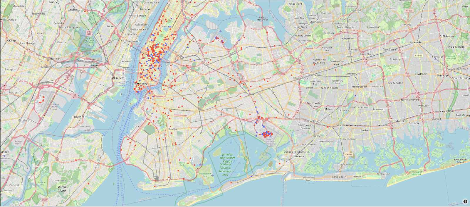
On close inspection of the plot, this cluster is associated with airport trips to and from JFK.
Scaling
Our previous example uses only a 3m row subset of the NYC taxi rides. Testing on a larger dataset for all of taxi rides for 2009 (170m rows), we can complete clustering for k=5 in around 3 mins with a ClickHouse service using 60 cores.
k=5
initializing...OK
…
Iteration 15, 16, 17, 18, 19
Number changed cluster in iteration 20: 288
stopping as moved less than 1000 clusters in last iteration
Execution time in seconds: 178.61135005950928
D^2 error for 5: 1839404623.265372
Completed in 178.61135005950928s and 20 iterations with error 1839404623.265372
This produces similar clusters to our previous smaller subset. Running the same clustering on a 64 core m5d.16xlarge using scikit-learn takes 6132s, over 34x slower! Steps to reproduce this benchmark can be found at the end of the notebook and using these steps for scikit-learn.
Potential improvements & future work
Clustering is very sensitive to the initial points selected. K-Means++ is an improvement over standard K-Means clustering that addresses this by introducing a smarter initialization process that aims to spread out the initial centroids, reducing the likelihood of poor initial centroid placement and leading to faster convergence as well as potentially better clustering. We leave this as an exercise for the reader to improve.
K-Means also struggles to handle categorical variables. This can be partially handled with one-hot encoding (also possible in SQL) as well as dedicated algorithms such as KModes clustering designed for this class of data. Custom distance functions for specific domains instead of just Euclidean distance are also common and should be implementable using User Defined Functions (UDFs).
Finally, it might also be interesting to explore other soft clustering algorithms, such as Gaussian Mixture Models for normally distributed features, or Hierarchical Clustering algorithms, such as Agglomerative clustering. These latter approaches also overcome one of the main limitations of K-Means - the need to specify K. We would love to see attempts to implement these in ClickHouse SQL!